An acousto-optic modulator (AOM) uses sound to control light. A radio-frequency (RF) signal drives a piezoelectric transducer, and the acoustic wave it launches strains the waveguide and changes its refractive index. On-chip AOMs are built for microwave signal processing, optical frequency shifting and microwave-to-optical conversion in quantum systems. Their closest relative, the electro-optic modulator (EOM), changes the index directly with the RF electric field. A thin-film lithium niobate EOM is broadband, from DC to tens of gigahertz, but its half-wave voltage-length product VπL is typically above 2 V·cm. An AOM works only in a narrow band around its acoustic resonance, but there its VπL can be several times lower and the device far shorter.
In this article, we demonstrate the design of a push-pull AOM on thin-film lithium niobate (TFLN) using both Flexcompute products and an open source acoustics solver. The design reaches a simulated VπL of 0.48 V·cm at 0.861 GHz, for a mechanical quality factor of 200.
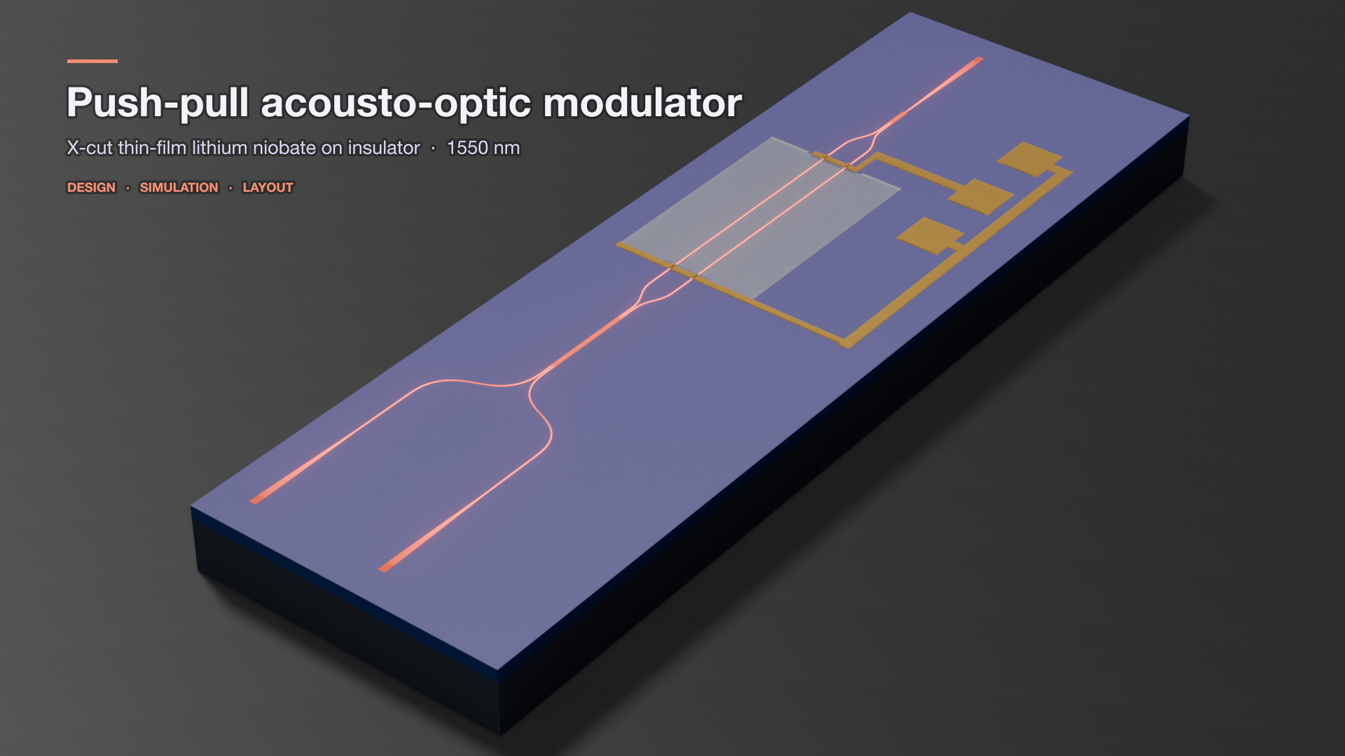
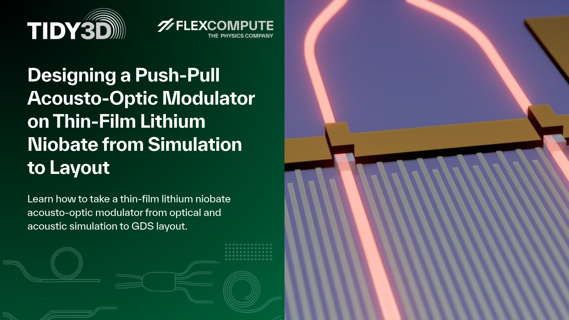
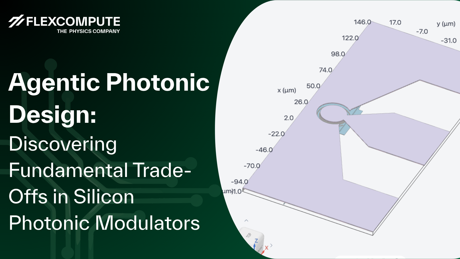
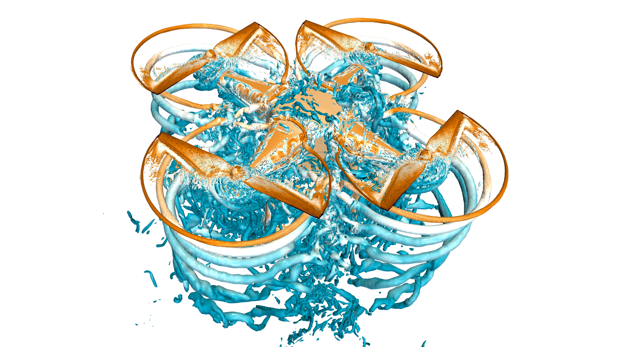
3D rendering of the designed AOM.
TFLN is a great platform for on-chip AOM because it is strongly piezoelectric and also a low-loss optical platform. Designing one is a multiphysics problem. The complex coupling between acoustics and optics needs to be carefully analyzed and optimized. Here we used Tidy3D for the optics, the open-source finite-element library NGSolve for the acoustics, and PhotonForge for the layout.
The device
The modulator is a Mach-Zehnder interferometer whose two arms pass through one surface-acoustic-wave transducer. An interdigital transducer launches a shear-horizontal acoustic wave across both arms. The arms sit 21 finger pitches apart, an odd number of half wavelengths, so the strain in one arm is always opposite to the strain in the other. One arm's index rises while the other's falls. This push-pull operation doubles the phase difference for a given drive voltage.
The concept, layer stack and transducer dimensions follow Ni, Bhave and Xu:
| Element | Design value |
|---|---|
| Film | X-cut lithium niobate, 360 nm, on 4.7 µm buried oxide on silicon |
| Rib waveguide | 2.0 µm wide, 180 nm etch |
| Transducer | Aluminium fingers at 2.2 µm pitch, 400 µm aperture, 40 reflector strips per side |
| Optical circuit | Grating couplers, 1×2 MMI, two arms, 2×2 MMI |
| Light | 1550 nm, TE polarization |
Step 1: the optical mode
The rib waveguide guides a TE0 mode with an effective index of 1.840 at 1550 nm. We computed it with the Tidy3D mode solver, which takes the full anisotropic permittivity of X-cut lithium niobate. The solve runs locally in seconds.
The same solver settled a layout question: how close may the aluminium fingers come to the arms? With two finger positions left empty around each arm, metal absorption is 0.05 dB/cm. With only one left empty it is 97 dB/cm, or 3.9 dB over the 400 µm aperture.
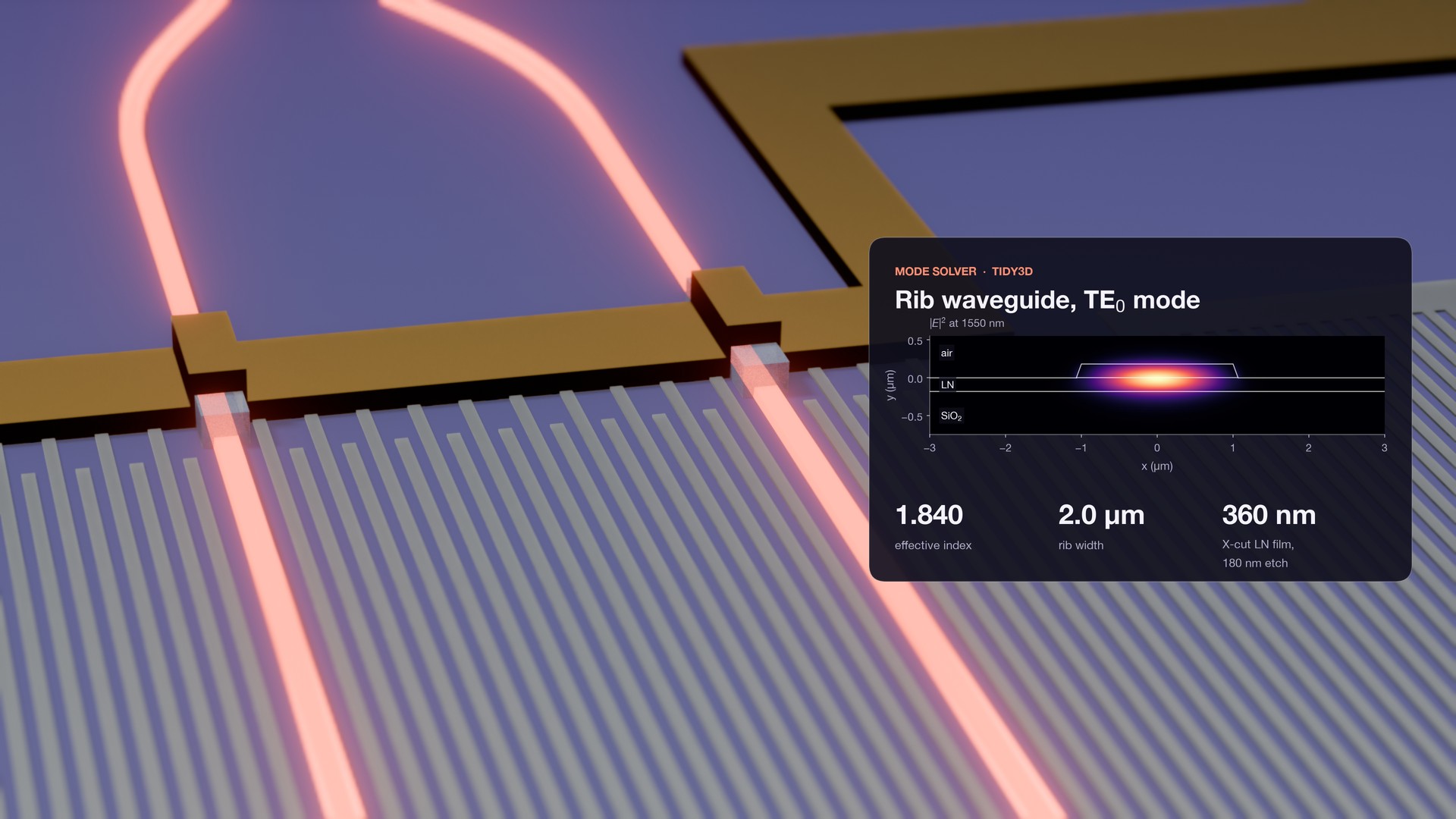
The two arms under the signal busbar, with the simulated TE0 mode.
Step 2: the acoustic wave and its overlap with the light
The transducer drives a shear-horizontal (SH0) wave whose acousto-optic response peaks at 0.861 GHz. A two-dimensional piezoelectric finite-element model of the full transducer cross-section gives the admittance and the strain field at each frequency. It has 1.1 million unknowns and covers the fingers, the reflectors, the oxide and the silicon, with absorbing regions at the edges. The 125 frequency points ran locally in about 20 minutes.
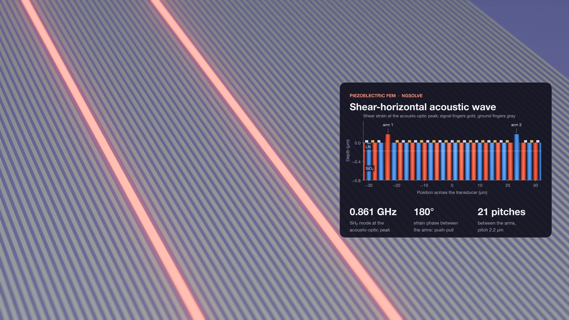
Shear strain at the acousto-optic peak. The two arms see strain of opposite sign.
Both the strain and the piezoelectric field change the optical permittivity: the strain through the photoelastic effect, the field through the electro-optic effect. An overlap integral with the optical mode from Step 1 turns them into an index change per volt in each arm. The two arms come out equal in size and 180° apart, as the push-pull layout intends.
The electro-optic term opposes the photoelastic one and is 30% of its size. Leaving it out would overstate the performance: 0.34 V·cm instead of 0.48 V·cm. A direct Tidy3D mode solve with the perturbed permittivity agrees with the overlap integral within 1%.
One input is uncertain: the mechanical quality factor of the film stack, Qm. We ran three values instead of picking one.
| Qm | S11 at resonance | VπL | Modulation linewidth |
|---|---|---|---|
| 100 | −15.3 dB | 0.63 V·cm | 16.9 MHz |
| 200 | −38.2 dB | 0.48 V·cm | 12.8 MHz |
| 400 | −16.7 dB | 0.41 V·cm | 11.3 MHz |
At Qm = 200 the transducer is matched to 50 Ω, and Vπ is 12.1 V for the 400 µm aperture. The photoelastic constant p14 is the other soft input: a 20% change moves VπL between 0.39 and 0.65 V·cm.
Step 3: splitters and couplers
The two MMIs were optimized with eigenmode expansion (EME) and the grating coupler with FDTD.
EME solves the modes of each cross-section once, so a length sweep of the MMI body costs almost nothing extra. The 1×2 splitter is 38.25 µm long with 0.03 dB excess loss. The 2×2 coupler is 155.47 µm long, splits 49.8 : 49.8, loses 0.02 dB, and delivers the 90° phase between its outputs.
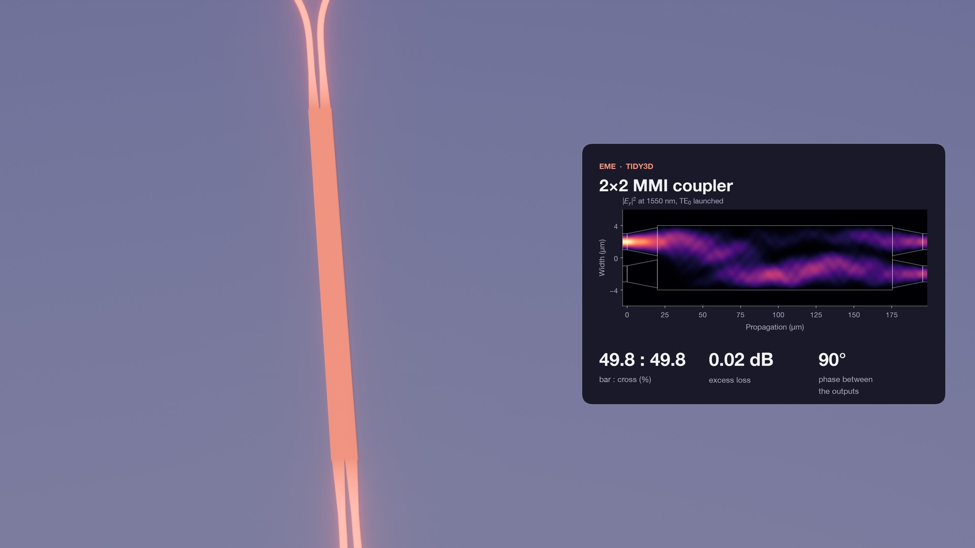
The 2×2 MMI with its simulated field, light launched in one input.
The grating coupler is a uniform grating with a 0.992 µm period, simulated in 2D FDTD. A row of Gaussian overlap monitors reads the coupling at 21 fiber positions in a single run. The coupler reaches −3.13 dB at 1550 nm into a fiber tilted 10°, with a 55 nm 1 dB bandwidth.
The power budget explains that number. Of the launched light, 57% radiates upward and 34% goes down into the substrate, and the upward beam overlaps the fiber mode by 86%.
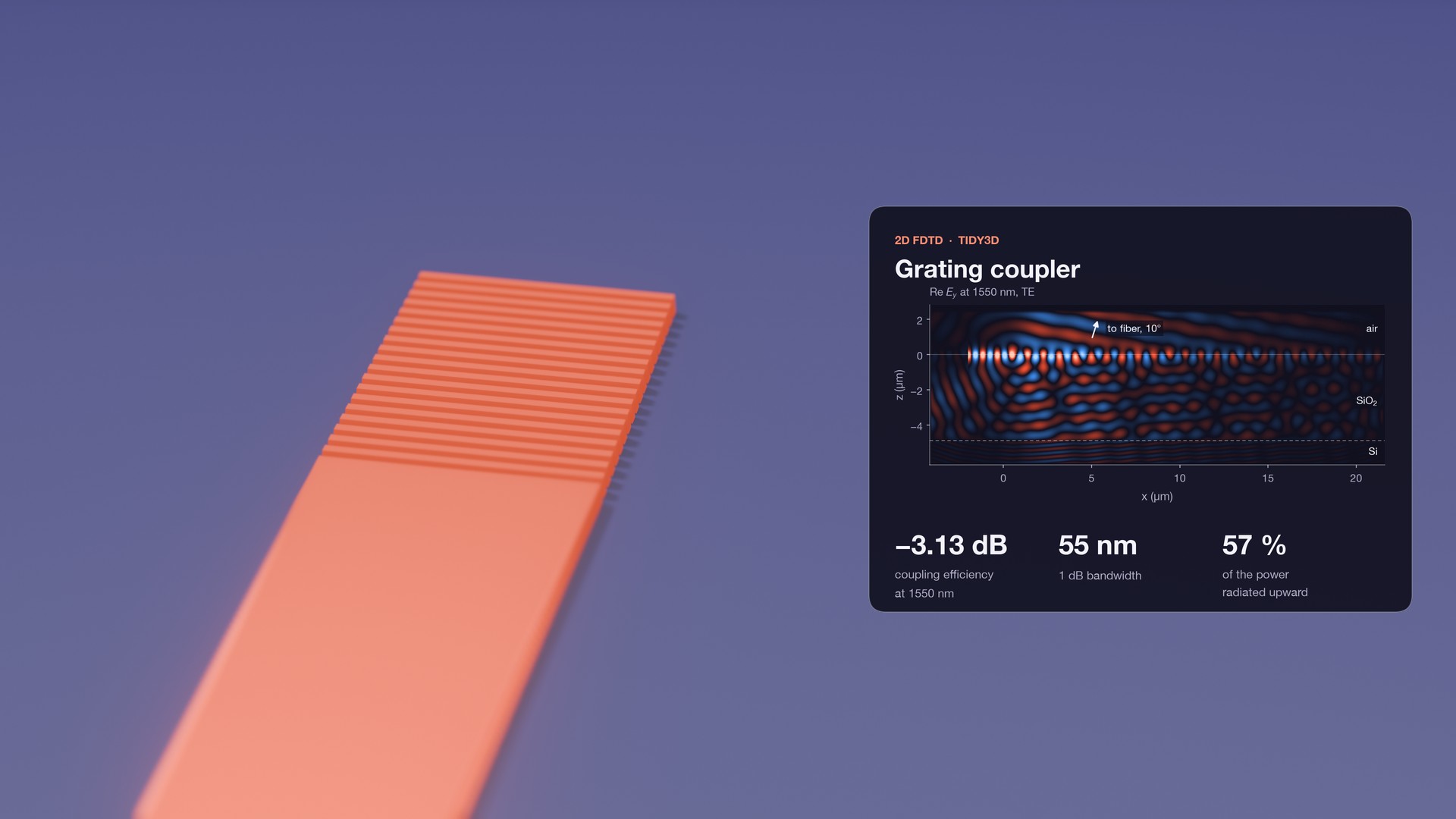
The input grating coupler with its simulated field cross-section.
Step 4: layout
PhotonForge turns the simulated dimensions into a GDS file. Parametric cells build the MMIs, the grating couplers and the transducer with its busbars and ground-signal-ground pads. The circuit measures 0.47 mm by 1.73 mm in footprint.
The transducer has 20 signal and 19 ground fingers between two sets of 40 reflector strips. Where a gold busbar crosses a waveguide, an oxide pad lifts the metal off the rib.
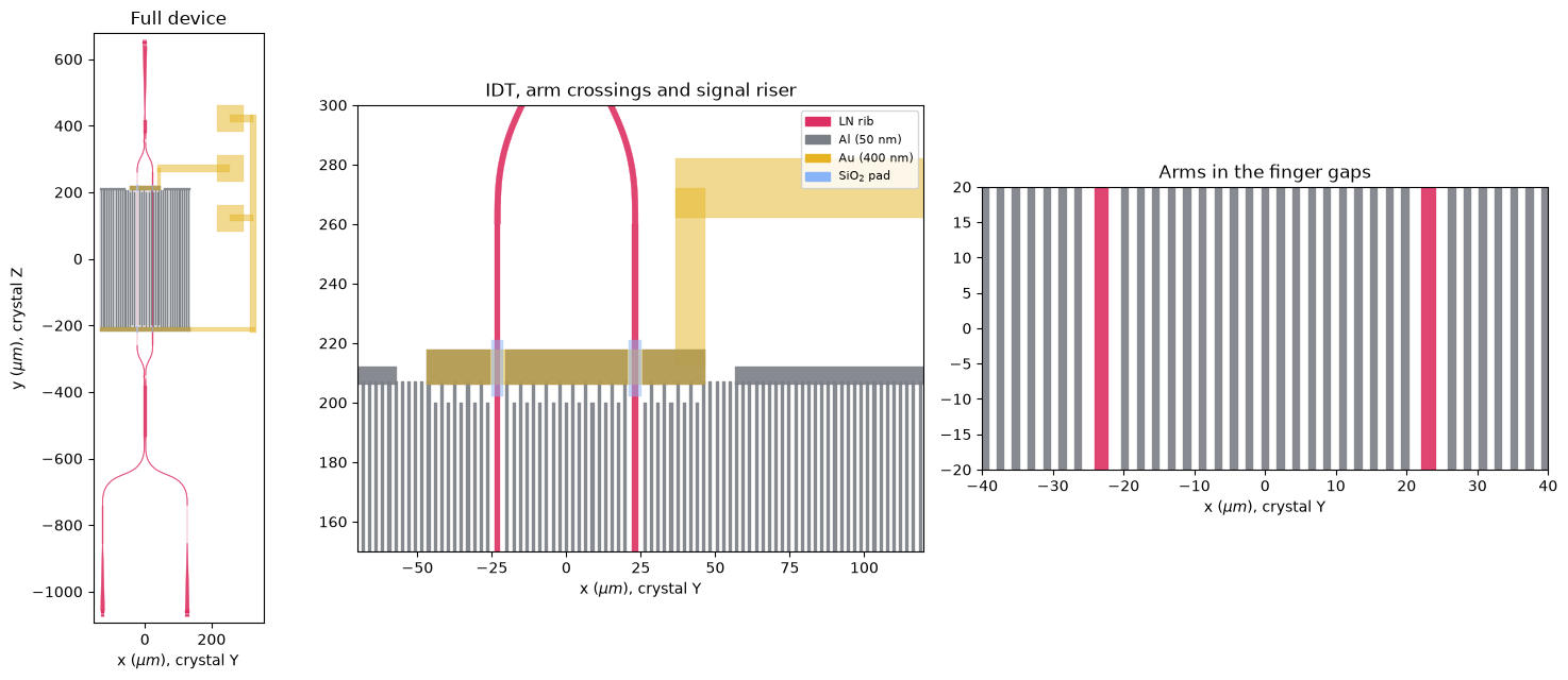
The layout: the full device, the signal busbar crossing the arms on oxide pads, and the arms in the finger gaps.
Results at a glance
The design reaches VπL = 0.48 V·cm with a matched transducer and low-loss passive optics, if Qm is 200.
| Quantity | Simulated value | Solver |
|---|---|---|
| VπL | 0.48 V·cm at Qm = 200 (0.41 to 0.63 for Qm = 400 to 100) | Piezoelectric FEM and mode overlap |
| Vπ | 12.1 V with a 400 µm aperture | Piezoelectric FEM and mode overlap |
| Acoustic frequency | 0.861 GHz, SH0 mode | Piezoelectric FEM |
| Electrical match | S11 = −38 dB at Qm = 200 | Piezoelectric FEM |
| Modulation linewidth | 12.8 MHz | Piezoelectric FEM |
| MMI excess loss | 0.03 dB (1×2) and 0.02 dB (2×2) | Tidy3D EME |
| Grating coupler | −3.13 dB per facet, 55 nm bandwidth | Tidy3D FDTD |
The Tidy3D cloud runs were estimated at under 7 FlexCredits in total. The acoustic sweeps ran locally.
Some elements are drawn but not simulated: the four waveguide crossings under the busbars, the S-bends, the grating tapers, and the pads and probe. The acoustic model is two-dimensional, so it leaves out diffraction along the finite fingers. The layout has no bias element for the interferometer yet.
Two inputs dominate the uncertainty in VπL: Qm and the photoelastic constant p14.
How it was built with an AI agent in the loop
An AI coding agent (Opus 5.5) in Flexcompute Agentic Design Environment (ADE) ran this workflow under an engineer's direction. It wrote the simulation code, ran the solvers, read the results, and produced the attached notebook, the layout and the figures in this post. The engineer chose the device, set the rules and approved the cloud runs.
Try it
The notebook below covers every step above, from the material tensors to the GDS.