Optical circuit switches (OCS) have had a busy autumn. In September, iPronics raised a $125 million Series B, with NVIDIA in the round, for its rack-mounted silicon photonics switch (optics.org). In October, Salience Labs closed its own $125 million round after showing a 64-port all-optical switch (Techzine). Two weeks later, the quantum computing company PsiQuantum unveiled an 8×8 OCS for AI data centers (The Quantum Insider). New startups are joining in, such as Dipole Labs, a Y Combinator company building optical switching for GPU clusters (RuntimeWire).

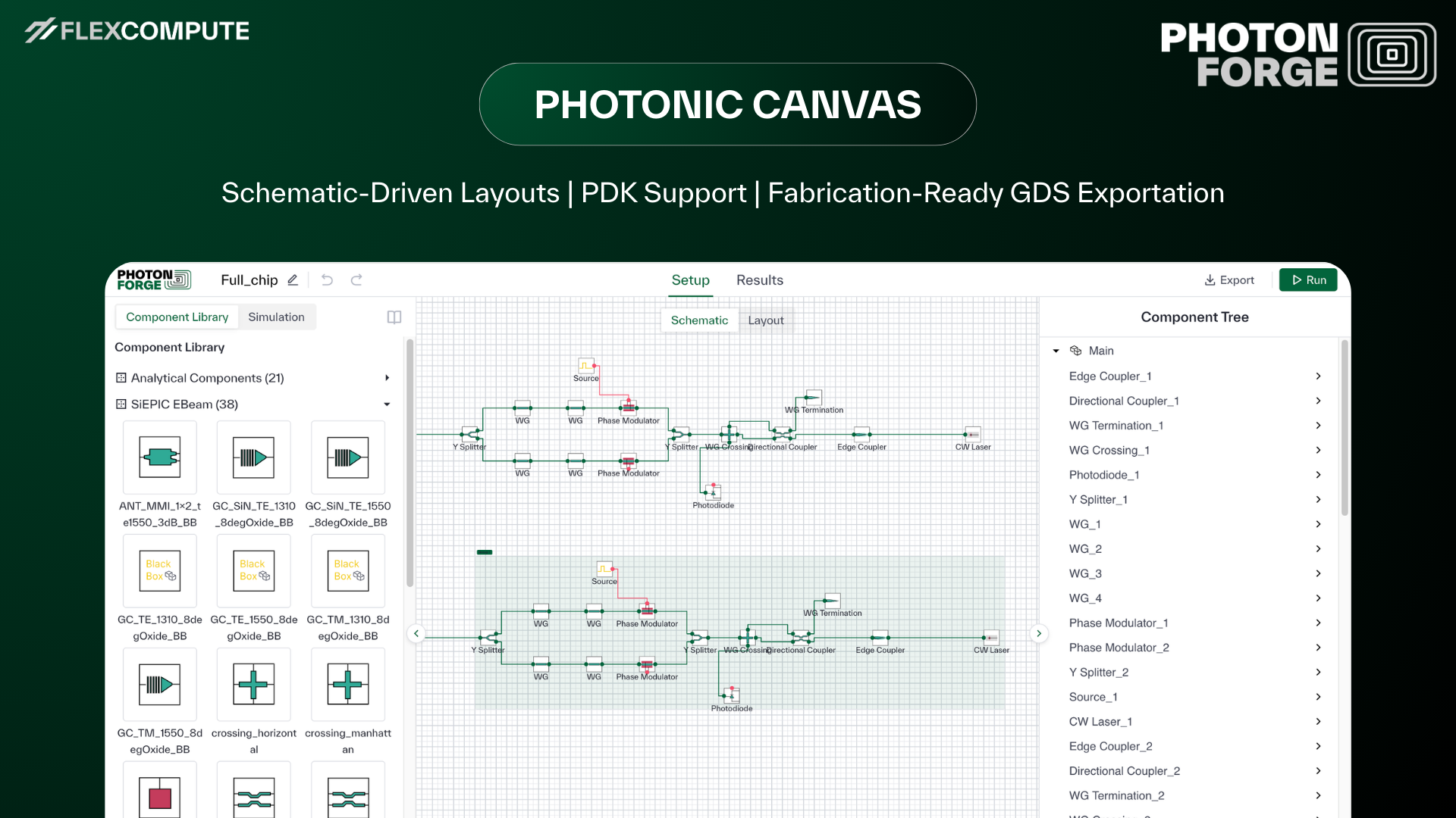
This article shows how to design an OCS with Flexcompute's Tidy3D and PhotonForge, using the example of a 4×4 silicon photonic switch meant to work without calibration. Tidy3D ran the physics simulations (mode solver, FDTD, EME and thermal), and PhotonForge ran the circuit simulation and created the full GDS layout.

What an optical circuit switch does

In a conventional data center network, data crosses several layers of electrical packet switches, and each one turns light into an electrical signal and back. An OCS skips that conversion. It connects an input fiber to an output fiber with a light path and holds it while traffic flows, at any data rate.

Google runs OCSes at scale. In its Jupiter network an OCS layer replaced the spine of electrical switches, and Google reports 40% less power and 30% less cost (Google Cloud blog). In its TPU v4 supercomputer, OCSes rewire the links between 4,096 chips for under 5% of the system's cost (TPU v4, ISCA 2023).

AI training put OCS back in the news, because the traffic between accelerators follows a pattern known in advance. Google steers light with MEMS mirrors, while iPronics, Salience Labs and PsiQuantum build their switches in silicon photonics. A common way to do that is a network of small 2×2 switches on one chip.

4×4 OCS design in Tidy3D and PhotonForge

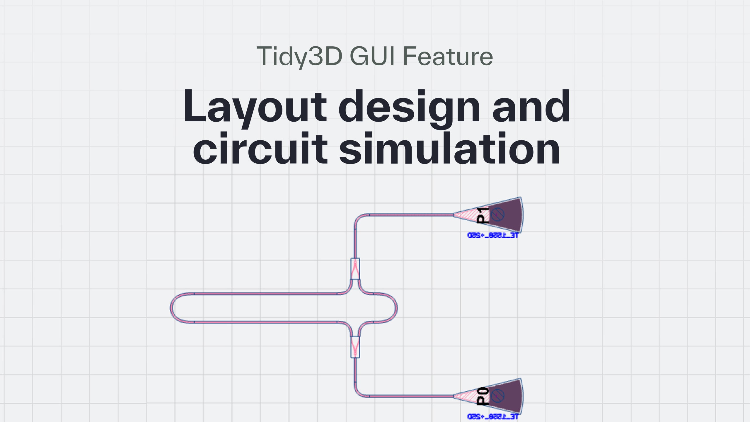
The designed switch is a 4×4 Benes network of six 2×2 Mach–Zehnder switches (MZSs) in three stages. Each MZS (Figure 1) splits the light in a multimode interference (MMI) coupler, sends it through two arms under TiN heaters, and recombines it in a second MMI. With the heaters off the light leaves by the cross port, and heating one arm until its phase shifts by π sends it to the bar port.

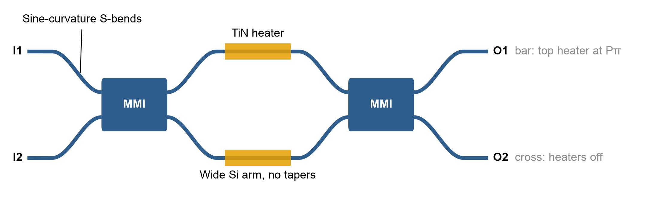
Figure 1. The 2×2 Mach–Zehnder switch. Light entering I1 leaves at O2 with the heaters off (cross) and at O1 when the top heater shifts its arm's phase by π (bar).

In a fabricated switch the two arms are never exactly equal, so each switch normally has to be measured and given a heater bias. That calibration grows with the fabric: a 64×64 Benes network has 352 switches. Song et al. proposed avoiding it with wide arms, whose effective index barely depends on width (Photonics Research 10, 793, 2022). We follow the same principle here, for TE light in silicon-on-insulator over 1520–1580 nm.

Step 1: choose the arm width with the mode solver

Everything starts from how fast the TE0 effective index changes with waveguide width (Figure 2). Tidy3D's mode solver can compute it locally at no cost (or in the cloud for a small cost). In an arm about four times as wide as a typical single-mode waveguide, ∂n_eff/∂w is 80 times smaller, so a few nanometers of width error barely move the arm phase.

The price is that a wide arm also guides TE1, TE2 and higher modes. Every bend or junction that excites them adds loss and crosstalk.

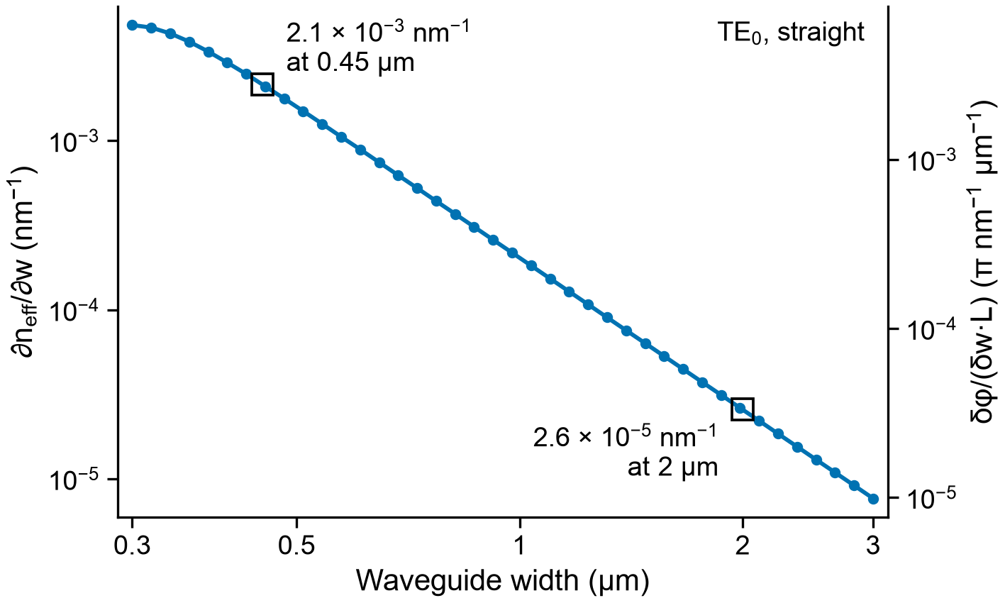
Figure 2. Width sensitivity of the TE0 effective index of a straight silicon strip, from the Tidy3D mode solver. The right axis gives the phase error per nm of width mismatch per µm of arm.

Step 2: design the bends and the MMI with FDTD and EME

Narrow sections are where width errors hurt most, so the arms stay wide from MMI to MMI, with no tapers. The fan-out uses S-bends whose curvature follows a sine: zero at both ends and at the inflection, so there is no curvature jump to excite TE1. A 3D FDTD sweep in Tidy3D set the bend length where the TE1 it excites cancels, and that bend loses at most 0.008 dB over the band.

The MMI sets the switch's extinction ratio (ER) at the band edges. Its even and odd self-images come to a focus at slightly different lengths, which tilts the 90° phase across the band, and the tilt shrinks as the MMI gets wider and longer. We screened about 60 geometries with Tidy3D's EME solver, which makes length sweeps nearly free, and set the length of the best one with 3D FDTD (Figure 3b, c).

The chosen MMI has access guides as wide as the arms. It loses 0.04 dB at 1550 nm and at most 0.19 dB over the band. Light from one input leaves as two equal images, 90° apart in phase (Figure 3a).

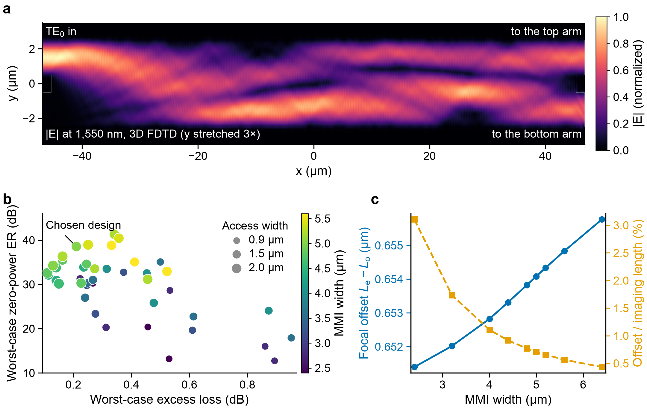
Figure 3. (a) |E| at 1550 nm in the chosen MMI from 3D FDTD, with TE0 entering the top input (y stretched 3×). (b) EME screen of MMI geometries: worst-case zero-power ER of an MZI against worst-case excess loss over 1520–1580 nm. Color gives the MMI width, and marker size the access width. (c) Distance between the even and odd focal planes (left) and its share of the imaging length (right).

Step 3: assemble the 2×2 switch in PhotonForge

We drew the switch with PhotonForge parametric components (Figure 4) and simulated it with PhotonForge's CircuitModel, which cascades the FDTD S-matrices with TE0, TE1 and TE2 on every wide port. Keeping TE2 matters: on an earlier variant, a full-device 3D FDTD showed that a circuit without it underestimated the loss by up to 0.08 dB. TE2 also sets the phase-shifter length, which we chose where the worst-case loss over the band is lowest.

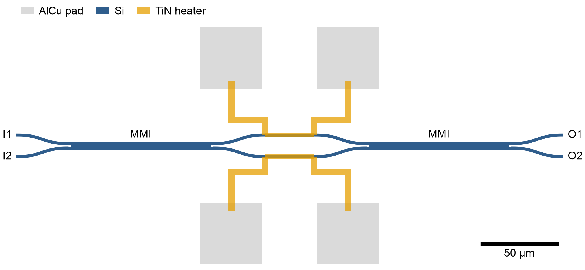
Figure 4. The 2×2 MZS in PhotonForge: two MMIs, wide S-bends and two TiN phase shifters with AlCu pads.

For the heater, a 2D thermal simulation in Tidy3D is sufficient. The arm phase depends only on the temperature integrated along the arm, which a 2D cross-section gives exactly for a straight arm (Figure 5a). It predicts a Pπ, the power for a π phase shift, of 25.8 mW.

The switch loses 0.10 dB at 1550 nm in the Off state and 0.11 dB in the On state, and at most 0.26 and 0.34 dB over the band. Its ER is 40.6 dB at 1550 nm and at least 32.7 dB over the band in the Off state, and 58.4 and 42.9 dB in the On state (Figure 5).

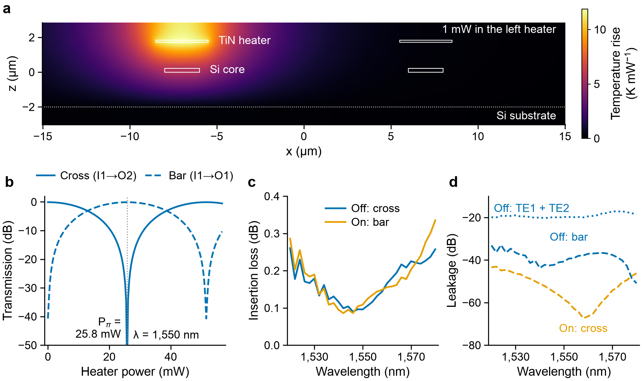
Figure 5. Heater and switching of the 2×2. (a) Temperature rise per mW in the cross-section, with 1 mW in the left heater, from a Tidy3D thermal simulation. (b) Transmission against heater power at 1550 nm. (c) Insertion loss in the Off (0 mW) and On (Pπ) states. (d) Leakage into the other port in each state, and the power left in TE1 and TE2 in the Off state.

Finally, we ran the whole switch as one 3D FDTD simulation of 3.1 billion cells (Figure 6) to validate the circuit simulation result. The light takes the path the circuit predicts. In the Off state the full device loses 0.08 dB at 1550 nm, against 0.10 dB from the circuit, and the cross port also agrees within 0.03 dB over the band.

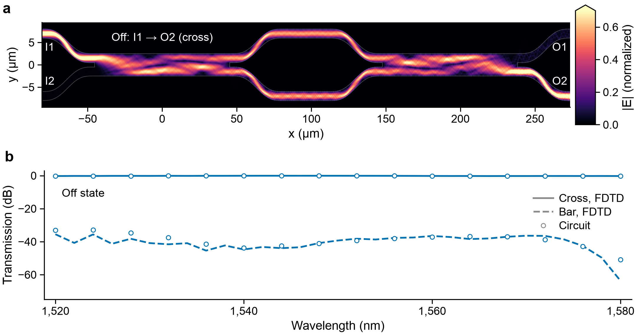
Figure 6. The whole 2×2 switch in one 3D FDTD run. (a) |E| at 1550 nm in the core mid-plane in the Off state, with TE0 entering I1 (y stretched 3×). (b) Transmission to the cross and bar ports from the full-device FDTD (lines) and from the circuit model (circles).

Step 4: check that it works without calibration

We gave the two arms of 400 switches a random width mismatch, at two levels estimated from the phase spreads Song et al. measured on fabricated switches. With the arm sensitivity from FDTD, the median zero-power ER at 1550 nm is 33.9 dB at the larger spread and 37.6 dB at the smaller one (Figure 7). Even at the larger spread, nine in ten switches stay above 26 dB with no heater bias at all.

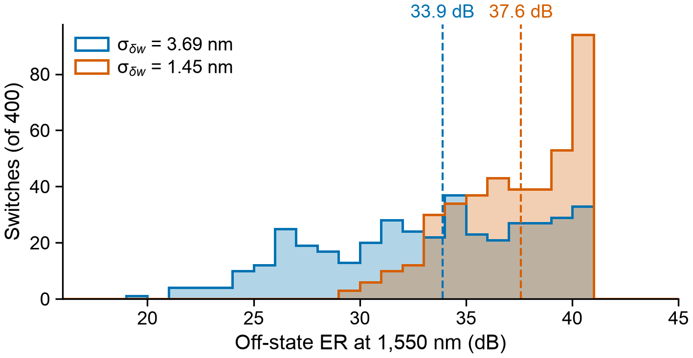
Figure 7. Zero-power ER at 1550 nm of 400 uncalibrated 2×2 switches with random arm-width mismatch. Dashed lines mark the medians.

Step 5: build the 4×4 fabric

We placed six switches in three stages and routed the shuffles in PhotonForge, with tapers down to single-mode links and an MMI-style crossing tuned in FDTD to 0.043 dB of loss and at most −43 dB of crosstalk (Figure 8).

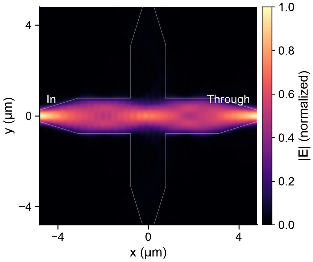
Figure 8. |E| at 1550 nm in the MMI-style crossing from 3D FDTD, with TE0 entering from the left. The light goes straight through, and the side arms stay dark.

PhotonForge's netlist drives the circuit simulation. With every heater off (all-cross), the fabric loses 0.40 dB at 1550 nm and 0.94 dB at worst over the band, with a worst-case ER of 28.8 dB (Figure 9). Without calibration, the median ER of its worst output is 26.0 dB at 1550 nm at the larger width spread.

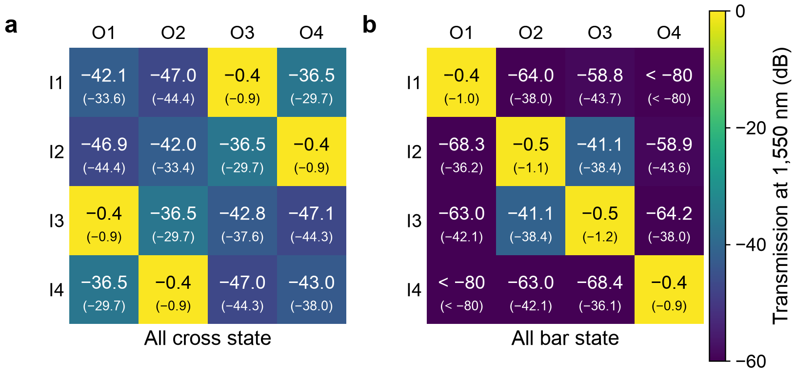
Figure 9. Transmission of the 4×4 from each input to each output at 1550 nm in the (a) all-cross and (b) all-bar states, with the worst value over 1520–1580 nm in brackets. Paths that need two leaks fall below −80 dB. Circuit model of the full layout.

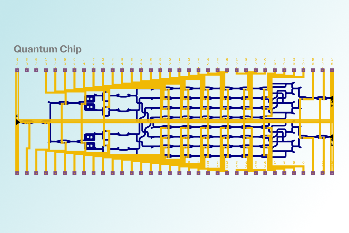
Figure 10 shows the complete chip, with all six switches and the heaters.

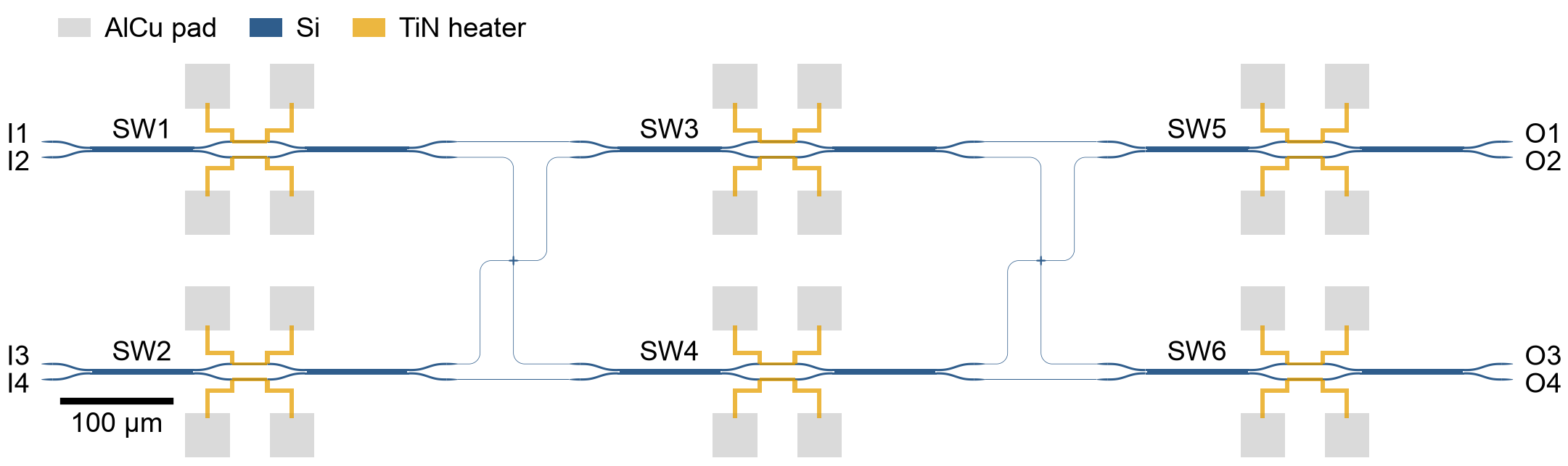
Figure 10. The full 4×4 Benes chip, drawn in PhotonForge: six MZSs (SW1–SW6) in three stages, one crossing in each shuffle, and AlCu pads for the 12 heaters.

Summary

The design ran end to end in Tidy3D and PhotonForge. In Tidy3D, the mode solver set the arm width and EME screened the MMI geometries. 3D FDTD then simulated the S-bends, MMI, crossing and taper, and a thermal simulation gave the heater power needed to switch. PhotonForge drew each component as a parametric cell and assembled the 2×2 switch and the 4×4 fabric. Its circuit simulations gave the switching performance. The Monte Carlo analysis shows the switches tolerate the expected width mismatch without calibration. The remaining limit is the MMI, which loses up to 0.19 dB at the band edges. Paired with agentic AI, designs like this can be done very efficiently: an AI agent ran this whole design in both tools, from the first mode solve to the final GDS.

The notebook below runs the whole design, from the mode solver to the final GDS.

Notebook: ocs_end_to_end.ipynb · Layout: ocs_4x4.gds

Sources

• iPronics Series B: optics.org, 3 September 2026

• Salience Labs funding round: Techzine, 14 October 2026

• PsiQuantum 8×8 OCS: The Quantum Insider, 28 October 2026

• Dipole Labs: RuntimeWire, 19 September 2026 and its Y Combinator page

• Google's OCS in Jupiter: The evolution of Google's Jupiter data center network, Google Cloud blog, 23 August 2022

• TPU v4: An Optically Reconfigurable Supercomputer for Machine Learning with Hardware Support for Embeddings, ISCA 2023

• L. Song et al., Toward calibration-free Mach–Zehnder switches for next-generation silicon photonics, Photonics Research 10, 793 (2022)