


import matplotlib.pyplot as plt
import numpy as np
import tidy3d as td
from tidy3d import web
TIDY3D
LEARNING CENTER
Example Library

Radiative losses analysis with ModeSimulation
ModeSimulation can be used to simulate small radiative losses, without the need for a full FDTD simulation. Since these losses are often very small (on the order of \(10^{-5}\) dB/cm), careful tuning of the parameters is necessary to ensure good convergence.
In this notebook, we will benchmark the required parameters to accurately calculate the imaginary part of the effective index for two types of losses: substrate leakage and bend losses.
For more information about ModeSimulation, refer to this tutorial.
Substrate leakage losses
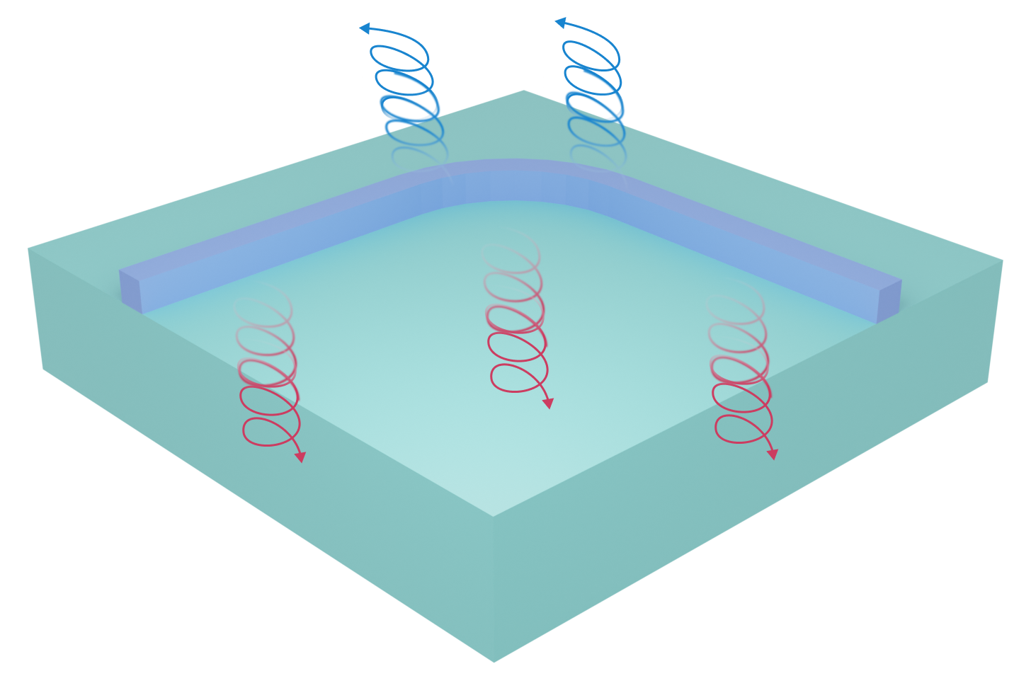
In this example, we will simulate radiative losses into the substrate for a strip waveguide fabricated in SOI, where the SiO₂ layer is thin enough to allow losses into the Si layer.
We will compare our results with the ones obtained in the paper of P. Bienstman, S. Selleri, L. Rosa, H. P. Uranus, W. C. L. Hopman, R. Costa, A. Melloni, L. C. Andreani, J. P. Hugonin, P. Lalanne, D. Pinto, S. S. A. Obayya, M. Dems, and K. Panajotov, "Modelling leaky photonic wires: A mode solver comparison", Optical and Quantum Electronics 38:731–759, (2006). DOI: 10.1007/s11082-006-9025-9, where the authors benchmarked the radiative losses of the structure depicted above, using different numerical methods.
Defining the simulation domain
We start defining a function for creating the ModeSimulation object.
Since we are interested in losses, some attributes must be carefully defined.
-
The default boundary condition (BC) for the
ModeSimulationobject is PEC. To study losses, we need to define a PML layer. This requires adding a tuple to thenum_pmlargument of theModeSpecobject, specifying the number of PML layers in each plane dimension.Note that the PML is added inside the simulation plane, so it is necessary to ensure that the simulation plane is large enough to prevent the PML from being too close to the structures. A good way to check this is by calling the
ModeSimulation.plot()method. To study low losses, we set the
precisionargument todouble, so the results will have more than six significant digits.
# defining the function for creating the ModeSimulation object


def mode_solver_substrate_loss(
    resolution,
    npml,
    delta_override=None,
    size=(3, 4.3),
    num_modes=3,
    target_neff=2.41,
    fields=["Ex", "Ey", "Ez"],
):
    # waveguide structure
    wg = td.Structure(
        geometry=td.Box(size=(td.inf, 0.5, 0.22)),
        medium=td.Medium(permittivity=3.5**2),
    )

    # SiO2 layer
    box = td.Structure(
        geometry=td.Box.from_bounds(rmin=(-td.inf, -td.inf, -100), rmax=(td.inf, td.inf, -0.11)),
        medium=td.Medium(permittivity=1.45**2),
    )

    # Si substrate
    substrate = td.Structure(
        geometry=td.Box.from_bounds(rmin=(-td.inf, -td.inf, -100), rmax=(td.inf, td.inf, -1.11)),
        medium=td.Medium(permittivity=3.5**2),
    )

    # mesh override region
    if delta_override:
        mesh_override = [
            td.MeshOverrideStructure(
                geometry=td.Box(center=(0, 0, 0), size=(0, 1.5, 1)),
                dl=(delta_override,) * 3,
            )
        ]
    else:
        mesh_override = []

    grid_spec = td.GridSpec.auto(
        min_steps_per_wvl=resolution, wavelength=1.55, override_structures=mesh_override
    )

    sim = td.Simulation(
        size=(4, size[0], size[1]),
        grid_spec=grid_spec,
        structures=[wg, box, substrate],
        run_time=1e-12,
        boundary_spec=td.BoundarySpec.all_sides(boundary=td.PML()),
        symmetry=(0, -1, 0),
    )

    mode_spec = td.ModeSpec(
        num_modes=num_modes,
        target_neff=target_neff,
        num_pml=(npml, npml),
        precision="double",
    )

    mode_solver = td.ModeSimulation.from_simulation(
        simulation=sim,
        plane=td.Box.from_bounds(
            rmin=(0, -size[0] / 2, -((size[1] - 0.3) / 2 + 0.3)),
            rmax=(0, size[0] / 2, 2 + (size[1] - 0.3) / 2),
        ),
        mode_spec=mode_spec,
        freqs=[td.C_0 / 1.55],
        fields=fields,
    )
    return mode_solver
# visualizing the mode simulation
mode_solver = mode_solver_substrate_loss(
resolution=20,
npml=9,
delta_override=None,
)
mode_solver.plot()
plt.show()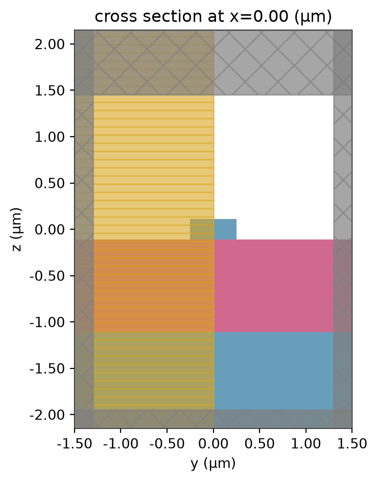
Next, we run the mode simulation to analyze the modes:
# run the mode simulation
mode_sim_data = web.run(mode_solver)
mode_data = mode_sim_data.modes
14:04:55 UTC Created task 'mode_2026-07-12_14-04-55' with resource_id 'mos-21712121-210e-429a-8c68-e036960319b7' and task_type 'MODE'.
14:04:57 UTC Estimated FlexCredit cost: 0.004. For this solver type, the
             estimate is the final billed cost.
14:04:58 UTC status = success
14:04:59 UTC Loading results from simulation_data.hdf5
# plot the fields
for i in range(mode_solver.mode_spec.num_modes):
    mode_sim_data.plot_field("E", "abs", mode_index=i)

plt.show()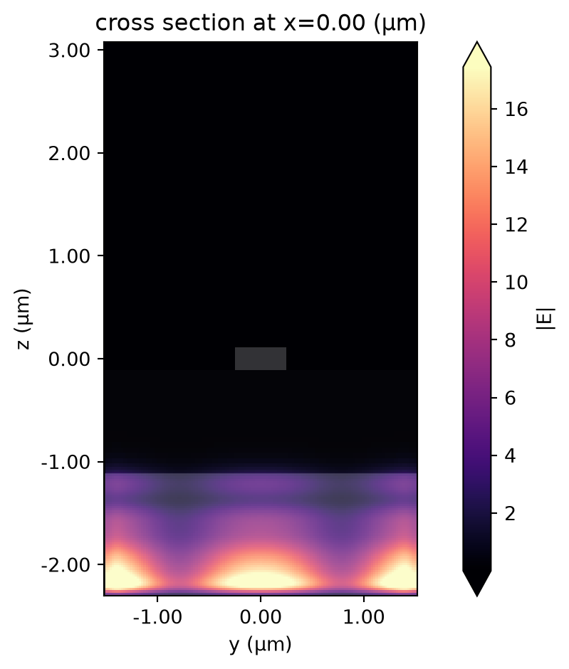
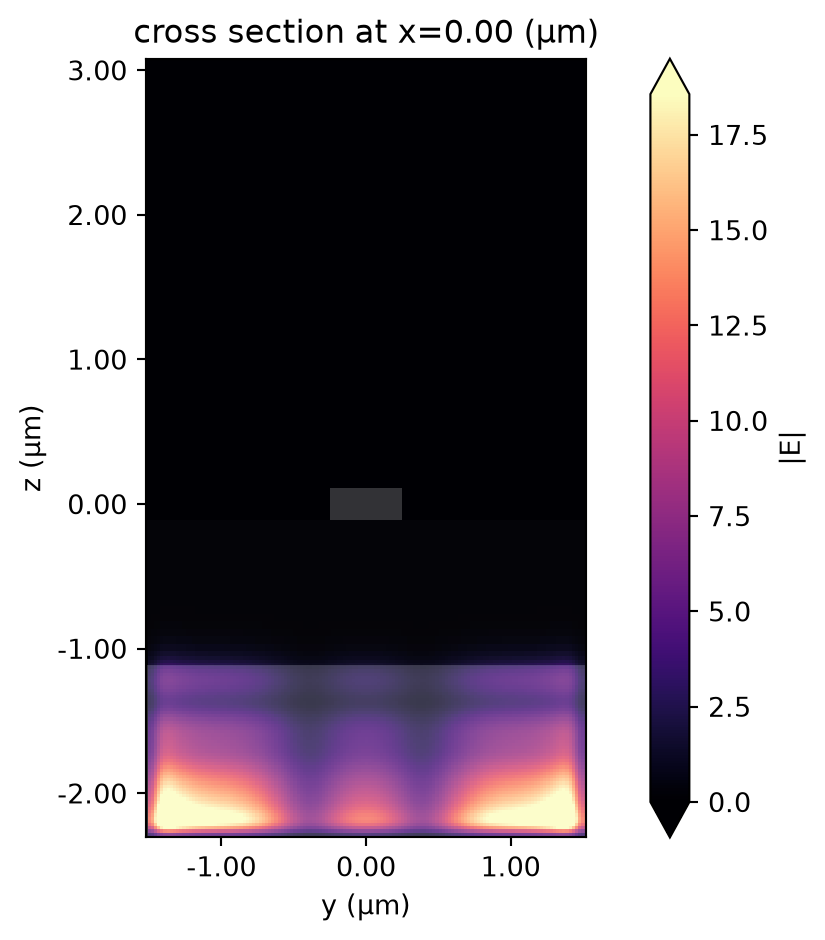
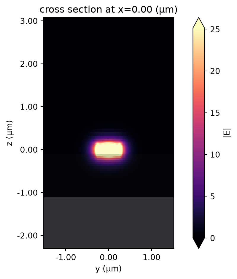
As one can note, the use of PMLs can lead to non-physical solutions. In this particular case, the physical mode is only the third one. Hence, when dealing with lossy structures, where PMLs are needed, it is important to carefully analyze the fields to exclude the non-physical ones. One way to achieve this is by looking at the effective index, which is approximately 2.4 for the real mode. Hence, we can just look at the mode closest to this value:
mode_data.to_dataframe()

 TERMS & CONDITIONS


 How the process works:
 Try this real URL to see an example: